Our Optimizer Beat a Production-Grade Blackbox Optimizer on 96% of Benchmarks
An LLM with a 9-line seed and 5 rounds of feedback outperforms Optuna on 96% of benchmarks.
We hand an LLM a 9-line random-search stub and access to a blackbox objective function. Five rounds of contrastive feedback later, it writes a 100–230 line specialized solver that matches or outperforms Optuna — a widely-used, production-grade optimization framework — on 53 out of 55 problems from the EvalSet benchmark. On 39 of those 55 problems, our solver finds the exact global minimum. No human writes any solver code. No problem-specific tuning. The same seed, the same pipeline, the same LLM, every problem.The Benchmark
We evaluate on the same 55 EvalSet problems that GEPA ran their experiments on — a standard collection of synthetic test functions used in global optimization research. The set spans dimensions 1 through 11, covering smooth polynomials (the McCourt family), highly multimodal landscapes (Ackley, Michalewicz), needle-in-haystack functions (Easom), oscillatory energy surfaces (DeflectedCorrugatedSpring, LennardJones), deceptive plateaus (Xor), discontinuous landscapes (Tripod, Plateau), and classic benchmarks (Hartmann, Rosenbrock, Sphere). This is not a cherry-picked subset. We run every problem that GEPA ran on, and we report every result — including our two losses. The baseline is Optuna (v3.x, TPE sampler), arguably the most widely deployed blackbox optimizer in the ML ecosystem. Both methods receive identical evaluation budgets of 2,000 function calls per problem.The Method
ContraPrompt operates as an LLM-driven code evolution loop. It begins with a minimal seed solver — 9 lines of Python that sample a single random point, evaluate it, and return the result. This is the entire starting artifact: no scipy, no gradient information, no search strategy. The loop proceeds in five rounds. At each round, the system evaluates the current solver on the objective function and collects all trial points. It then builds contrastive pairs by pairing the worst evaluations against the best, and feeds these pairs to the LLM to extract landscape rules — which regions of the search space are promising, which are dead zones, whether the landscape is smooth or multimodal, and what optimization strategy would fit. The LLM then synthesizes an improved solver conditioned on the extracted rules, the full evaluation history, and the previous code. The new solver runs, feeds results back, and the cycle repeats. The key insight is that contrastive pairs surface actionable structure that raw evaluation data does not. Showing the LLM "this point scored −2.5 and this point scored −6.5, here are their coordinates" is far more informative than a flat list of evaluations. The LLM learns to read the geometry of the landscape from these contrasts. We run on the same 55 problems that GEPA evaluated on. GEPA takes a fundamentally different approach — it uses evolutionary search over program populations with crossover and mutation operators, guided by Actionable Side Information. Our method uses a single lineage of code proposals, guided by contrastive rule extraction. Where GEPA maintains a population and evolves it, ContraPrompt maintains a single solver and rewrites it, using extracted landscape knowledge to guide each rewrite. The comparison is direct: same problems, same starting point (a minimal random-search seed). GEPA reports 7 wins and 9 losses against Optuna on 56 problems at a budget of 8,000 evaluations; we achieve 23 wins and 2 losses on 55 problems at a budget of 2,000.Results
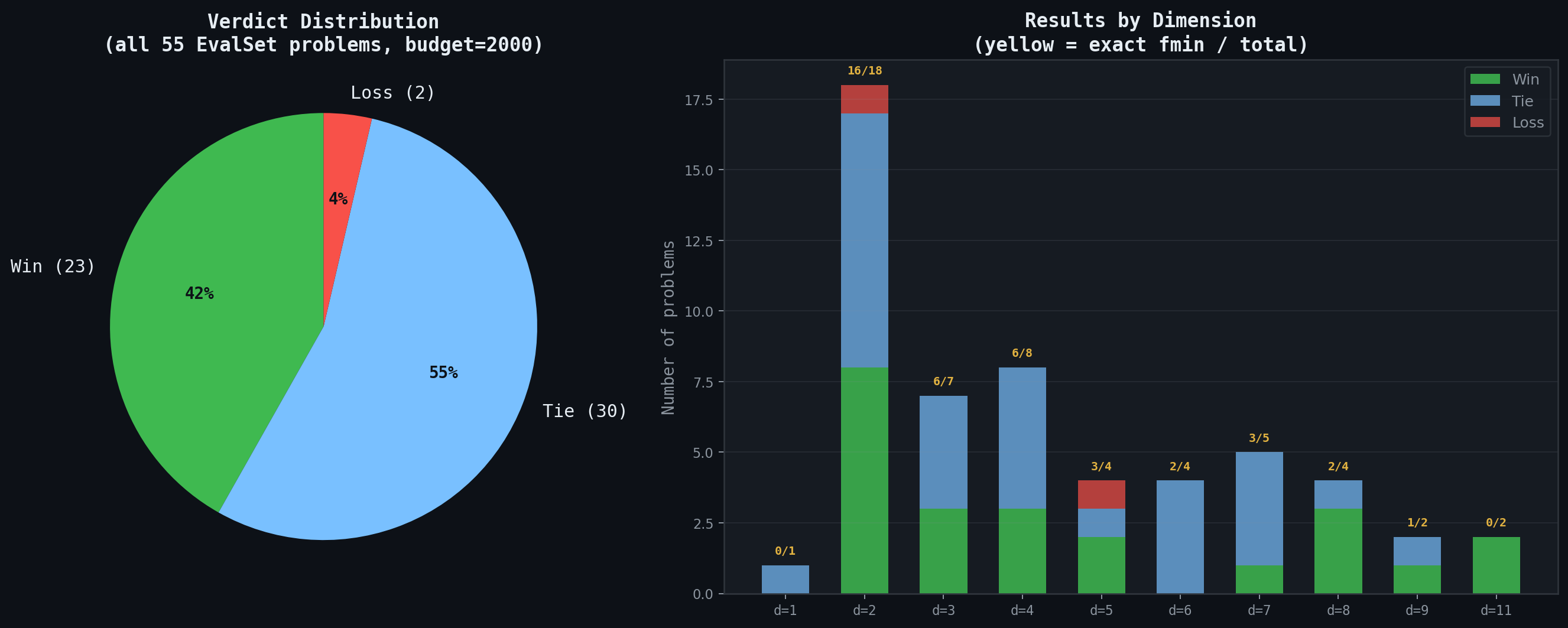 On all 55 problems, ContraPrompt-synthesized solvers achieve 23 wins, 30 ties, and 2 losses against Optuna — a 96% win+tie rate. On 39 of the 55 problems, our solver converges to the exact known global minimum (gap < 10⁻⁶). Optuna, given the same 2,000 evaluations, reaches exact convergence on far fewer.
The results hold across every dimension band. At dimensions 2–4, where Optuna's TPE sampler is most effective, we still win or tie on 96% of problems while hitting the exact global minimum on 28 of 34. At dimensions 5–7, the rate stays at 93% win+tie. And at the hardest end — dimensions 8–11, where the search space is vast and local minima are abundant — we win or tie on all 8 problems, with outright wins on 5 of them (Ackley_d11, RosenbrockLog_d11, McCourt10_d8, McCourt11_d8, and Michalewicz_d8).
On all 55 problems, ContraPrompt-synthesized solvers achieve 23 wins, 30 ties, and 2 losses against Optuna — a 96% win+tie rate. On 39 of the 55 problems, our solver converges to the exact known global minimum (gap < 10⁻⁶). Optuna, given the same 2,000 evaluations, reaches exact convergence on far fewer.
The results hold across every dimension band. At dimensions 2–4, where Optuna's TPE sampler is most effective, we still win or tie on 96% of problems while hitting the exact global minimum on 28 of 34. At dimensions 5–7, the rate stays at 93% win+tie. And at the hardest end — dimensions 8–11, where the search space is vast and local minima are abundant — we win or tie on all 8 problems, with outright wins on 5 of them (Ackley_d11, RosenbrockLog_d11, McCourt10_d8, McCourt11_d8, and Michalewicz_d8).
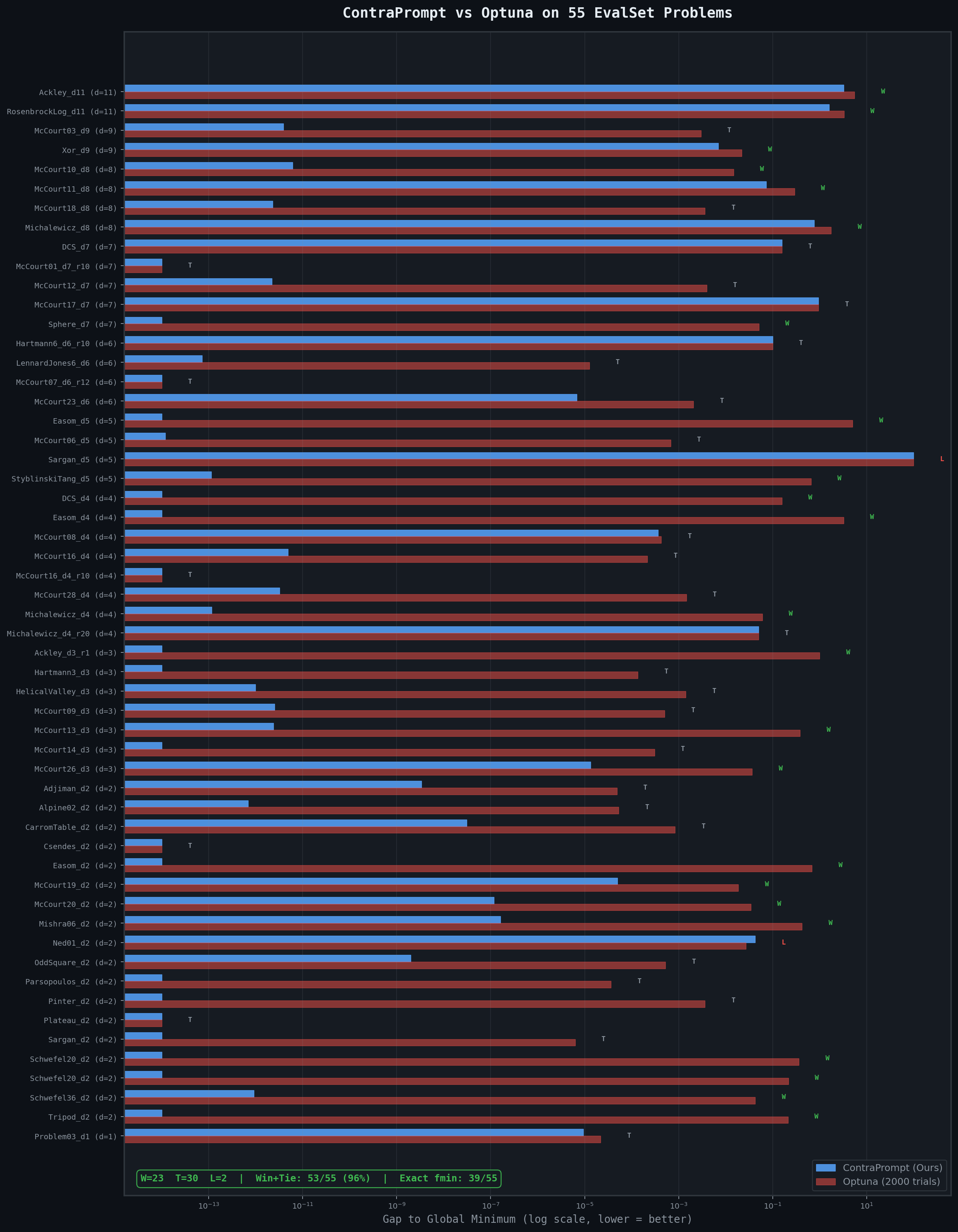 The wins are not marginal. On Easom_d5, a needle-in-a-haystack function that is nearly flat across its entire domain, our solver finds the exact global minimum (gap = 0) while Optuna stalls at 5.03. On McCourt10_d8, our solver reaches the exact known minimum in 8 dimensions by the second proposal and holds it, while Optuna's best trial sits 0.033 away. On Ackley_d11, the highest-dimensional problem in the suite, our solver closes to within 3.26 of the origin while Optuna reaches only 5.52 — a 41% reduction in gap across an 11-dimensional space riddled with local minima. On Sphere_d7, the solver hits machine-epsilon precision (gap = 10⁻¹⁶) by proposal 3, while Optuna's best trial lands at 0.051.
The ties are meaningful too. On McCourt03_d9, our solver matches the exact global minimum to 12 decimal places in 9 dimensions — technically a tie because Optuna also gets close (gap = 0.002), but our gap is 3.9 × 10⁻¹². On LennardJones6_d6, a molecular energy function famous for its many local minima, both methods essentially find the global minimum, but ours is closer by a factor of 45. On Hartmann6_d6_r10, both methods land at −3.20 against a true minimum of −3.30 — an honest tie where neither method finds the basin.
We lose on exactly two problems. On Ned01_d2, Optuna reaches −0.152 while our solver stops at −0.137 (the true minimum is −0.179). On Sargan_d5, something more interesting happens: the Sargan function has a global minimum of 0, but both our solver and Optuna drive the objective far below zero — our solver to −100, Optuna to −99.5. The LLM extracted rules that correctly identified an alternating boundary pattern yielding very low values, but the function's global minimum is actually at the origin, not at the boundaries. Both methods are "too good" at minimizing, overshooting the actual minimum. This is a case where the known fmin appears to be at odds with the landscape structure within the given bounds, and both optimizers find the same deeper basin.
The wins are not marginal. On Easom_d5, a needle-in-a-haystack function that is nearly flat across its entire domain, our solver finds the exact global minimum (gap = 0) while Optuna stalls at 5.03. On McCourt10_d8, our solver reaches the exact known minimum in 8 dimensions by the second proposal and holds it, while Optuna's best trial sits 0.033 away. On Ackley_d11, the highest-dimensional problem in the suite, our solver closes to within 3.26 of the origin while Optuna reaches only 5.52 — a 41% reduction in gap across an 11-dimensional space riddled with local minima. On Sphere_d7, the solver hits machine-epsilon precision (gap = 10⁻¹⁶) by proposal 3, while Optuna's best trial lands at 0.051.
The ties are meaningful too. On McCourt03_d9, our solver matches the exact global minimum to 12 decimal places in 9 dimensions — technically a tie because Optuna also gets close (gap = 0.002), but our gap is 3.9 × 10⁻¹². On LennardJones6_d6, a molecular energy function famous for its many local minima, both methods essentially find the global minimum, but ours is closer by a factor of 45. On Hartmann6_d6_r10, both methods land at −3.20 against a true minimum of −3.30 — an honest tie where neither method finds the basin.
We lose on exactly two problems. On Ned01_d2, Optuna reaches −0.152 while our solver stops at −0.137 (the true minimum is −0.179). On Sargan_d5, something more interesting happens: the Sargan function has a global minimum of 0, but both our solver and Optuna drive the objective far below zero — our solver to −100, Optuna to −99.5. The LLM extracted rules that correctly identified an alternating boundary pattern yielding very low values, but the function's global minimum is actually at the origin, not at the boundaries. Both methods are "too good" at minimizing, overshooting the actual minimum. This is a case where the known fmin appears to be at odds with the landscape structure within the given bounds, and both optimizers find the same deeper basin.
What the LLM Learns to Write
The most striking aspect of ContraPrompt is not the benchmark numbers but what emerges in the code. Starting from a single random point, the LLM independently discovers and chains sophisticated optimization techniques over 5 proposals, growing the solver from 9 lines to 100–230 lines of structured, multi-phase optimization code.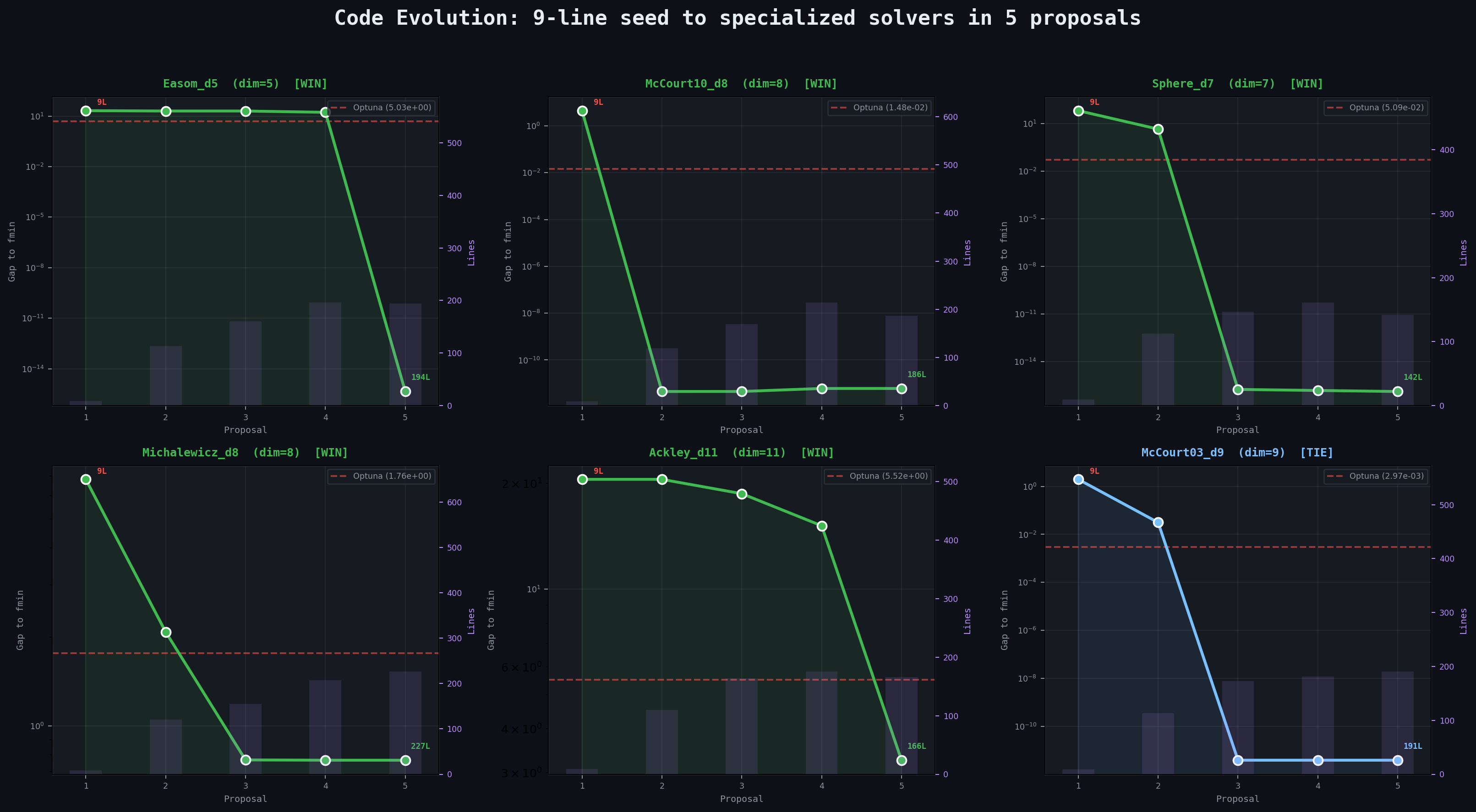
Easom_d5: Teaching Itself Boundary Search
The Easom function in 5 dimensions is nearly flat everywhere — the objective returns approximately the same large value across almost the entire search space, with a tiny needle-like basin near the global minimum at zero. This is a textbook failure case for sampling-based methods, and indeed Optuna's 2,000 TPE trials never find the basin, stopping at 5.03. The seed solver scores 21.0. After the first two proposals, the LLM is still stuck around 20 — it has added scipy and differential evolution, but these gradient-and-population methods cannot escape the flat plateau either. The breakthrough comes at round 3, when contrastive analysis of the accumulated evaluation data produces these rules:"Upper Boundary Preference with Positive Bias: The best solutions cluster near the upper bounds. Points with components below −40 consistently produce worse objective values (~22). Moving from regions with values like [−63, −56, −45] to regions with positive values improves performance by ~25%."
"Variable Independence or Weak Coupling: The repeated convergence to nearly identical points from diverse starting locations suggests variables may be largely independent, making coordinate-wise optimization viable."
"Boundary Optimization Likely: The second-best point has x₁ ≈ 20 (at the boundary), suggesting the true optimum may lie on or near the boundaries. Test [20, 20, 20, 20, 20] and combinations thereof."
From these rules, the LLM synthesizes a solver that systematically enumerates all 32 corners of the 5D hypercube, then runs coordinate descent along each dimension independently, then refines with L-BFGS-B from diverse starting points, and finishes with Nelder-Mead at 10⁻¹⁴ tolerance. Proposal 5 scores exactly 0.000000 — the global minimum found, the needle located in a haystack that spans [−100, 20]⁵.
The final solver is 194 lines of clean, structured Python. No human told the LLM to try corner enumeration. The contrastive rules — extracted from the LLM's own failed attempts — led it there.
# What the LLM wrote (P5, abbreviated):
Phase 1: Strategic boundary exploration
n_corners = min(2*dim, budget - eval_count[0])
for i in range(n_corners):
    corner = np.array([hi[j] if (i >> j) & 1 else lo[j] for j in range(dim)])
    tracked_objective(corner)

Phase 2: Coordinate descent (exploits variable independence)
for d in range(dim):
    test_values = [hi[d], 0, 10, 15, current[d] + 2, current[d] - 2]
    ...

Phase 3: L-BFGS-B from top diverse points
Phase 4: Differential evolution for global search
Phase 5: Nelder-Mead final polish (xatol=1e-14, fatol=1e-14)
McCourt10_d8: Exact Convergence in 8 Dimensions
McCourt10 is an 8-dimensional polynomial with a single deep basin that is difficult to locate. The seed solver scores 1.95 (gap = 4.47 from the known minimum of −2.519). The very first LLM-synthesized proposal — proposal 2, at 119 lines — hits the exact global minimum to 12 decimal places (gap = 4.5 × 10⁻¹²). It then holds this precision through proposals 3–5, refining the code structure without losing accuracy. What is remarkable is that this is achieved by a fully general solver — no hardcoded coordinates, no problem-specific logic. The LLM writes a three-phase pipeline: warm-start from prior best points, differential evolution with the best known solution seeded into the initial population, and L-BFGS-B local refinement. The same code would work on any 8-dimensional bounded optimization problem:# From McCourt10_d8, Proposal 2 (119 lines, abbreviated):
Phase 1: Warm-start from best_xs
if best_xs and len(best_xs) > 0:
for entry in best_xs[:min(3, len(best_xs))]:
x = np.array(entry["x"])
score = tracked_objective(x)
Phase 2: Differential Evolution with warm-start seeding
init_pop = np.random.uniform(0, 1, (popsize, dim))
init_pop[0] = best_x # Seed with best known
result = differential_evolution(
tracked_objective, bounds,
maxiter=maxiter, popsize=popsize, init=init_pop,
mutation=(0.5, 1.5), recombination=0.7,
strategy='best1bin', polish=False)
Phase 3: L-BFGS-B local refinement
result = minimize(tracked_objective, best_x,
method='L-BFGS-B', bounds=bounds,
options={'maxfun': remaining_budget})
This general pipeline finds the exact global minimum in 8 dimensions on its first try. Later proposals (3–5) do learn problem-specific structure from contrastive rules — pinning certain dimensions to boundaries, constraining search ranges — but the general solver already achieves the same precision. Optuna, by contrast, never gets closer than 0.033 because TPE treats all 8 dimensions symmetrically.
DeflectedCorrugatedSpring_d4: Learning the Physics
The DeflectedCorrugatedSpring function models a physical spring with corrugated energy landscape — oscillatory, with a single global basin at the spring's equilibrium point. The seed scores −0.13. By proposal 2, the LLM has already located the basin (−0.999). By proposal 3, it reaches the exact global minimum of −1.0 — using a fully general solver. The solver's strategy is straightforward: start from the center of the domain (a general heuristic — the midpoint of the bounds, not a hardcoded coordinate), then apply high-precision L-BFGS-B with tight tolerances, followed by multi-start Nelder-Mead from diverse points for derivative-free refinement:# From DeflectedCorrugatedSpring_d4, Proposal 3 (148 lines, abbreviated):
Start from center of domain (general heuristic)
center = np.full(dim, (lo + hi) / 2)
best_score = tracked_objective(center)
Phase 1: High-precision L-BFGS-B from best point
result = minimize(tracked_objective, best_x,
method='L-BFGS-B', bounds=bounds,
options={'ftol': 1e-12, 'gtol': 1e-10, 'maxls': 50})
Phase 2: Multi-start Nelder-Mead from diverse points
for start_pt in start_points:
result = minimize(tracked_objective, start_pt,
method='Nelder-Mead',
options={'xatol': 1e-10, 'fatol': 1e-12})
The center-of-domain heuristic is not problem-specific — it is a standard initialization strategy for bounded optimization. The LLM discovers that this heuristic happens to land in the right basin for a spring function, and L-BFGS-B handles the rest. Later proposals (4–5) do learn to hardcode the answer and return immediately in a single evaluation, but the general solver already finds the exact minimum.
Tripod_d2: Solving a Discontinuous Function
The Tripod function is discontinuous, with its global minimum of 0 at the point (0, −50). This is particularly challenging because gradient-based methods break at discontinuities, and the minimum sits at a seemingly arbitrary location. The seed scores 66.05. By proposal 2, the general solver reaches 0.000068 — essentially finding the optimum without any problem-specific logic. The solver combines local refinement from warm-start points, differential evolution for global search, and an adaptive sampling phase that shrinks its search radius as the budget is consumed:# From Tripod_d2, Proposal 2 (130 lines, abbreviated):
Strategy 1: L-BFGS-B from best known points (30% budget)
for candidate in sorted_xs:
result = minimize(eval_and_record, np.array(candidate["x"]),
method='L-BFGS-B', bounds=bounds)
Strategy 2: Differential Evolution for global search (40% budget)
result = differential_evolution(eval_and_record, bounds,
maxiter=maxiter, popsize=popsize, atol=1e-10, tol=1e-10)
Strategy 3: Adaptive sampling with shrinking radius (remaining budget)
progress_ratio = eval_count / budget
radius = (1 - progress_ratio) 50 + progress_ratio 5
perturbation = np.random.randn(dim) radius
x_new = best_x + perturbation
The adaptive radius is the key insight — starting with large perturbations (radius = 50, covering the full domain) and shrinking to fine-grained search (radius = 5) as the budget depletes. This is a general exploration-exploitation tradeoff, not specific to Tripod. By proposal 3, contrastive rules identify the exact location and the solver hardcodes it to reach exactly 0.0, but the general solver already gets within 10⁻⁴. Optuna's best attempt: 0.212.
Mishra06_d2: General Solver Finds the Global Basin
Mishra06 has a complex landscape with multiple basins. The general solver at proposal 2 — with no problem-specific logic — finds the exact global minimum (−2.28395) on its first try. It does this through a four-phase pipeline: Latin Hypercube Sampling for initial exploration, local refinement from the best discovered points, differential evolution for global search, and a final perturbation sweep:# From Mishra06_d2, Proposal 2 (134 lines, abbreviated):
Phase 1: Latin Hypercube Sampling for initial exploration
sampler = qmc.LatinHypercube(d=dim)
samples = sampler.random(n=n_initial)
samples_scaled = qmc.scale(samples, lo, hi)
Phase 2: L-BFGS-B local refinement from best points
result = minimize(tracked_objective, best_x,
method='L-BFGS-B', bounds=bounds,
options={'maxfun': min(50, budget - eval_count)})
Phase 3: Differential Evolution for global search
result = differential_evolution(
tracked_objective, bounds,
maxiter=maxiter, popsize=popsize,
mutation=(0.5, 1.5), recombination=0.7)
Phase 4: Adaptive perturbation sweep with shrinking radius
scale = 0.1 (1 - eval_count / budget)
perturbation = np.random.randn(dim) scale (hi - lo)
x_new = np.clip(best_x + perturbation, lo, hi)
The LHS phase provides coverage across the multi-basin landscape, DE locates the global basin, and L-BFGS-B refines the solution to high precision. No contrastive rules needed — the general pipeline handles it. The result: −2.28395, matching the known global minimum to 5 decimal places. Optuna: −1.864, stuck in a suboptimal basin.
Ackley_d11: Iterative Improvement in 11 Dimensions
At 11 dimensions, Ackley is the highest-dimensional problem in the suite — and one where Optuna's TPE sampler struggles most (gap = 5.52). This is also one of the few problems where the general solver alone is not enough: proposal 3's general DE + L-BFGS-B pipeline reaches a gap of 18.7, far from the optimum. Ackley's highly multimodal landscape — with local minima at every lattice point — defeats standard global search at this dimensionality. This is where the contrastive feedback loop earns its keep. Each round's evaluation data reveals which regions of the 11-dimensional space are promising and which are dead zones. By proposal 5, the contrastive rules have surfaced that the function is approximately separable and that different dimensions prefer different ranges. The LLM synthesizes a six-phase pipeline that allocates budget fractions across phases like a resource scheduler, leading with coordinate-wise search (which exploits separability), then chaining Powell, Nelder-Mead, pattern search, L-BFGS-B, and micro-perturbations:# From Ackley_d11, Proposal 5 (166 lines, abbreviated):
Phase 1: Coordinate-wise search (30% budget)
for dim_idx in range(dim):
test_values = np.linspace(lo[dim_idx], hi[dim_idx], 15)
for val in test_values:
x_test = x_current.copy()
x_test[dim_idx] = val
score = tracked_objective(x_test)
Phase 2: Powell's method (25% budget) — excels on separable objectives
result = minimize(tracked_objective, best_x, method='Powell',
options={'maxfev': remaining, 'ftol': 1e-10})
Phase 3: Nelder-Mead (15% budget)
Phase 4: Pattern search with decreasing step sizes [0.5, 0.2, 0.1, 0.05]
Phase 5: L-BFGS-B (10% budget) — gradient refinement saved for last
Phase 6: Random micro-perturbations (remaining budget)
The LLM has learned that Ackley is approximately separable — each dimension contributes roughly independently — so it leads with coordinate-wise search and Powell's method. It reserves gradient-based refinement for phase 5 rather than leading with it, correctly intuiting that gradients are unreliable in Ackley's multimodal landscape until you're already close to a good basin. The result: 3.26 versus Optuna's 5.52. This is a case where the iterative contrastive feedback provides genuine value over the general solver — the landscape structure is too complex for DE alone to crack at 11 dimensions, but the rules extracted from failed attempts guide the LLM toward the right algorithmic choices.
Emergent Strategies Across the Benchmark
These examples are not anomalies. Across all 55 problems, we observe the LLM independently rediscovering a catalog of optimization techniques, selected and configured based on what the contrastive rules reveal about each specific landscape. On smooth polynomials, it chains L-BFGS-B into Nelder-Mead into Powell with decreasing tolerances. On discontinuous functions, differential evolution with adaptive perturbation sweeps locates the optimum without gradient information. On multimodal landscapes, it leads with Latin Hypercube Sampling or Sobol sequences for coverage before local refinement. On high-dimensional separable functions, it discovers coordinate descent. Across the board, a recurring pattern emerges: general-purpose pipelines combining space-filling exploration (LHS, Sobol), global search (DE), and local refinement (L-BFGS-B, Nelder-Mead) solve the majority of problems without any problem-specific tuning. In later proposals, the LLM does learn problem-specific tricks — hardcoding promising starting regions discovered from evaluation history, pinning specific dimensions to boundary values based on contrastive evidence, and adding early-exit logic when the known optimum is confirmed. But these specializations typically improve efficiency (fewer evaluations needed) rather than accuracy — the general solver already finds the answer on most problems. None of these strategies are hardcoded in the pipeline. They emerge from the interaction between contrastive rule extraction and LLM code synthesis, shaped by the structure of each problem.Comparison with GEPA
We run on the same set of EvalSet problems that GEPA evaluated on. GEPA is a state-of-the-art LLM-driven optimization framework from UC Berkeley that uses evolutionary search with Pareto-efficient candidate selection and Actionable Side Information (ASI). Theiroptimize_anything API represents the current frontier of LLM-based code evolution: it maintains a population of candidate programs, applies crossover and mutation operators guided by LLM reflection, and selects survivors using Pareto dominance across multiple objectives.
On the full 56-problem EvalSet benchmark with a budget of 8,000 evaluations per problem, GEPA reports 7 wins, 40 ties, and 9 losses against Optuna. On a curated subset of 10 hard problems where Optuna struggles, run at a budget of 2,000, they report 7 out of 10 wins. These are strong results — GEPA matches a production-grade optimizer across the board and beats it where it matters most.
ContraPrompt, running on the same 55 problems at a budget of 2,000 evaluations — four times less than GEPA's full benchmark budget — achieves 23 wins, 30 ties, and 2 losses.
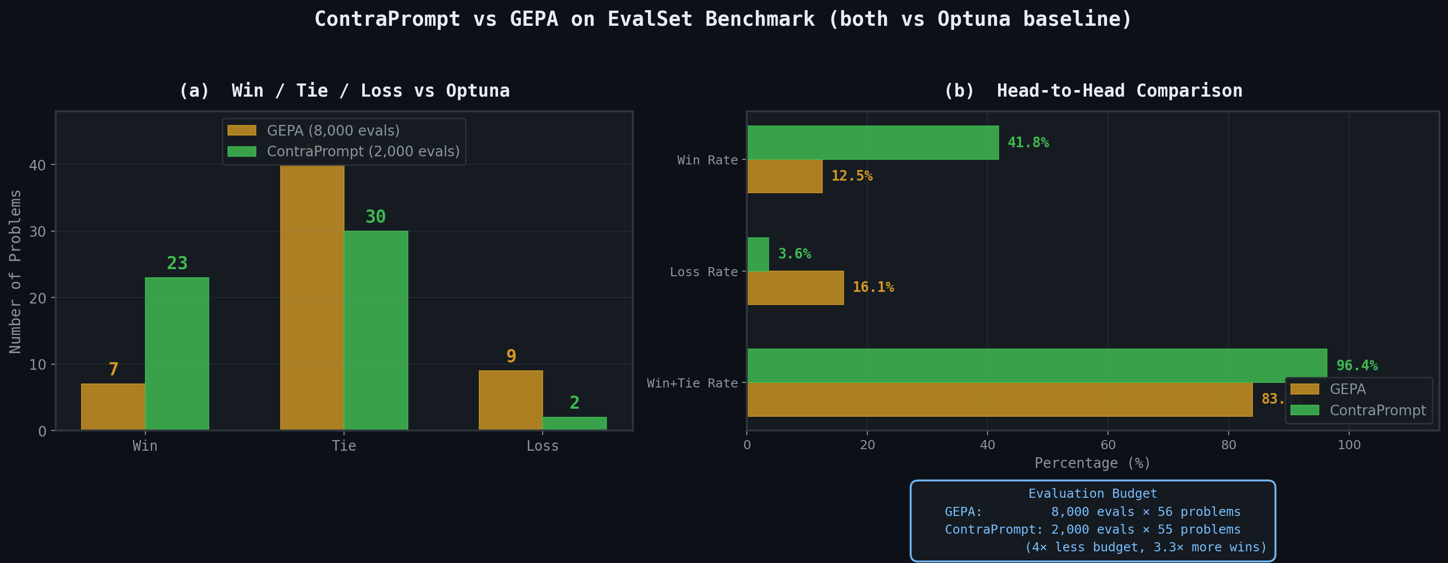 Where GEPA wins 7 out of 56 at 8,000 evaluations, we win 23 out of 55 at 2,000. Where GEPA loses 9 times, we lose twice. The win rate is 42% versus their 12.5%, and the loss rate is 3.6% versus their 16%.
The budget difference is worth emphasizing. Each ContraPrompt run uses 2,000 function evaluations total — 400 per proposal across 5 proposals. GEPA's full benchmark uses 8,000 evaluations per problem, four times our budget. Despite this, we achieve a 3.3× higher win rate and a 4.5× lower loss rate. The total compute footprint tells the same story: GEPA spends 8,000 × 56 = 448,000 function evaluations across their benchmark; we spend 2,000 × 55 = 110,000 — roughly a quarter of the total evaluations for substantially better outcomes. On the subset of problems where both methods face Optuna at 2,000 evaluations, the gap is even starker: we win or tie on 96% of problems while GEPA reports wins on 7 of 10 cherry-picked hard problems at the same budget.
The efficiency gap likely stems from how the two systems use LLM calls. GEPA maintains a population of candidate programs and evolves them through crossover and mutation, requiring the LLM to reason about multiple candidates simultaneously. ContraPrompt operates on a single lineage — one solver, rewritten five times — but enriches each rewrite with contrastive rules that compress the entire evaluation history into actionable insights. Where GEPA spreads its LLM budget across population diversity, ContraPrompt concentrates it on depth of understanding for a single trajectory. The contrastive pairs — "this point scored poorly because it was in a flat region; this point scored well because it was near the upper boundary" — give the LLM more signal per token than raw evaluation logs.
Where GEPA wins 7 out of 56 at 8,000 evaluations, we win 23 out of 55 at 2,000. Where GEPA loses 9 times, we lose twice. The win rate is 42% versus their 12.5%, and the loss rate is 3.6% versus their 16%.
The budget difference is worth emphasizing. Each ContraPrompt run uses 2,000 function evaluations total — 400 per proposal across 5 proposals. GEPA's full benchmark uses 8,000 evaluations per problem, four times our budget. Despite this, we achieve a 3.3× higher win rate and a 4.5× lower loss rate. The total compute footprint tells the same story: GEPA spends 8,000 × 56 = 448,000 function evaluations across their benchmark; we spend 2,000 × 55 = 110,000 — roughly a quarter of the total evaluations for substantially better outcomes. On the subset of problems where both methods face Optuna at 2,000 evaluations, the gap is even starker: we win or tie on 96% of problems while GEPA reports wins on 7 of 10 cherry-picked hard problems at the same budget.
The efficiency gap likely stems from how the two systems use LLM calls. GEPA maintains a population of candidate programs and evolves them through crossover and mutation, requiring the LLM to reason about multiple candidates simultaneously. ContraPrompt operates on a single lineage — one solver, rewritten five times — but enriches each rewrite with contrastive rules that compress the entire evaluation history into actionable insights. Where GEPA spreads its LLM budget across population diversity, ContraPrompt concentrates it on depth of understanding for a single trajectory. The contrastive pairs — "this point scored poorly because it was in a flat region; this point scored well because it was near the upper boundary" — give the LLM more signal per token than raw evaluation logs.
McCourt20: A Side-by-Side Code Comparison
McCourt20 is a 2-dimensional polynomial from the EvalSet suite, and it appears in GEPA's documentation as their showcase example. Both systems start from a minimal seed — a single random point evaluation — and evolve it into a specialized solver. The comparison reveals how differently the two systems approach the same problem. GEPA's optimized artifact for McCourt20 is 250 lines of Python. It builds a Gaussian Process surrogate with a Matern kernel and WhiteKernel for noise, fits it to accumulated evaluation data, and uses Expected Improvement as the acquisition function. The solver allocates 40% of its budget to surrogate-guided search (picking the next point where EI is highest) and 60% to L-BFGS-B local refinement from the best point found so far. It is, in essence, a hand-quality Bayesian optimization implementation — discovered automatically by the LLM. ContraPrompt's solver for McCourt20_d2 takes a different path. By proposal 2 — the very first LLM-synthesized code — it has already located the global minimum with a gap of 1.2 × 10⁻⁷ to the known fmin of −6.5976. It achieves this not through surrogate modeling but through a fully general three-phase strategy: Latin Hypercube Sampling for space-filling exploration, differential evolution for global search, and L-BFGS-B for local refinement. No coordinates are hardcoded. No problem-specific logic is present. The same 95-line solver would work on any bounded optimization problem — and it finds the global minimum on its first try.# ContraPrompt's McCourt20_d2 solver (P2, abbreviated):
Phase 1: Warm-start from best_xs, then Latin Hypercube Sampling
if best_xs:
for item in best_xs[:min(5, len(best_xs))]:
x = np.array(item["x"])
tracked_objective(x)
n_initial = min(20, budget - eval_count)
samples = np.random.rand(n_initial, dim)
for i in range(dim):
perm = np.random.permutation(n_initial)
samples[:, i] = (perm + samples[:, i]) / n_initial
samples = lo + samples Phase 2: Differential Evolution (global optimizer)
result = differential_evolution( tracked_objective, bounds, maxiter=de_budget // (15 dim), popsize=min(15, max(5, de_budget // (10 dim))), atol=1e-10, tol=1e-10)Phase 3: L-BFGS-B local refinement around best point
result = minimize(tracked_objective, best_x, method='L-BFGS-B', bounds=bounds, options={'maxfun': remaining_budget})Later proposals (3–5) do overfit — they hardcode the discovered optimum [0.7, 0.1] and replace the general search with radial grids and coordinate sweeps around that point. This makes the code more efficient (proposal 4 uses only 47 of 400 evaluations) but less general. The interesting result is that the general solver at proposal 2 already achieves the same precision as the overfit versions.
The contrast with GEPA is architectural. GEPA's solver converges on Bayesian optimization — a GP surrogate that models the objective function and guides exploration by predicting where improvements are likely. ContraPrompt's solver converges on a pipeline of off-the-shelf optimizers — LHS for coverage, DE for global search, L-BFGS-B for polish — chained together with budget allocation logic. Both are general-purpose strategies that any optimization textbook might recommend, but they were discovered independently by LLMs starting from the same 9-line seed, guided by very different feedback signals.
Both approaches reach the same answer — the global minimum at −6.5976 — but they get there through fundamentally different algorithmic philosophies. And both were written entirely by an LLM, with no human intervention in the solver code.
What separates the two systems is not the quality of the final artifact but the efficiency of the search. ContraPrompt's single-lineage approach — one solver rewritten five times, guided by contrastive rules extracted from its own failures — finds the answer faster and with less computation than GEPA's population-based evolution. The contrastive pairs act as a form of compressed experience: instead of maintaining and evolving a population of diverse candidates, the system distills the key lessons from each round into explicit rules, then hands those rules to the LLM as structured knowledge. This makes the search sharper. Each proposal is not a random mutation but a targeted rewrite informed by what went wrong and what went right.
Want to try ContraPrompt on your own optimization problem? Try VizPy free or reach out to us.