Prompt Optimization for Analog Circuit Placement
Prompt optimization reaches 97% of expert analog circuit placement quality — with zero training data.
Placement for analog circuit layout lacks the automated P&R flows available for digital design. Each transistor position affects matching, routing, and parasitics — expert layout engineers spend hours hand-tuning layouts using intuition built over years. We investigate whether prompt optimization methods can teach LLMs to perform this task, starting from zero domain-specific training data. We recently released VizPy and have been evaluating our prompt optimization methods across several use cases. Analog circuit placement proved to be a particularly demanding benchmark due to the tight coupling between spatial reasoning, connectivity analysis, and multi-objective optimization.Problem Formulation
Given a SPICE netlist (transistors, types, connectivity), produce (x, y) grid coordinates minimizing:score = 1.0 + (0.8 × wire_penalty + 0.2 × area_penalty)
Wire penalty (80% weight) measures total Manhattan distance between connected device centers. Area penalty (20%) measures bounding box size. No overlaps permitted. Expert placements score 0.65–0.70.
Our dataset consists of 9 differential amplifier variants (5 devices each), split 6/3 train/test. We note this is a small dataset — results should be interpreted with this constraint in mind. We also evaluate two unseen circuit families: CKTA (4-input NAND cascode, 8 devices) and CKTB (SR latch, 8 devices with cross-coupled feedback).
Baseline: Test-time RL Fine-tuning
Test-Time Training (TTT) — RL fine-tuning a 120B parameter model with PUCT tree search — memorized the training circuit (0.670, matching expert) but averaged 0.502 on test circuits, with a worst case of 0.385. The model learned specific coordinate patterns rather than transferable placement principles.ContraPrompt
ContraPrompt mines good-vs-bad output pairs, extracts rules via a reflection LM, and validates each rule individually before injection. We augmented the standard contrastive pairs with expert (ground truth) placements on the "good" side — rather than comparing the LLM's best vs. worst attempts, we compared the LLM's worst attempt against expert placement descriptions (structural patterns without specific coordinates, to avoid rules that memorize exact positions). Starting from 0.500 baseline, 3 iterations:- Iteration 1: 5 candidate rules extracted, 1 survived validation (4 degraded performance). Score: 0.596.
- Iteration 2: 5 more candidates, 3 survived. Score: 0.624.
- Iteration 3: 3 candidates extracted but the resulting prompt scored 0.535 — the optimizer correctly rejected this iteration.
The two surviving rules teach column-based layout with drain-pair alignment, discovered entirely from optimization feedback:
Rule 1: Prioritize column-based vertical stacking and structural relationships between devices sharing critical signal nets (drain-paired PMOS and NMOS on the same output nodes).
Rule 2: Separate PMOS and NMOS into distinct columns, enumerate drain-paired devices, and output a structured placement plan rather than stopping at topology understanding.
We expected the rules to encode specific numeric parameters (x-offsets, y-offsets). Instead, they encode high-level strategy — the LLM determines specific values at generation time based on each circuit's device dimensions.
Post-Optimization Code Generation
After prompt optimization with Sonnet, we generated placement code using Opus with the optimized prompt. The LLM produces a Python function that algorithmically computes placements — not raw coordinates but executable code evaluated across all training circuits. We selected the best code across 6 training circuit prompts based on cross-circuit evaluation (each candidate was scored on all 6 training circuits to enforce generality). Train average: 0.636 (expert 0.665, 96%). Test average: 0.634 (expert 0.652, 97%). On test_amp8, the generated code exceeds the expert (0.640 vs 0.626). On test_amp0, it matches exactly (0.670). No circuit scores below 0.604. A note on model capability: Opus produces similar code quality from the prompt alone — the ContraPrompt rules close a 24% gap for Sonnet but are largely redundant for Opus, which independently converges to the same column-based strategy. Code generation is a constrained output space; the function contract and helper API narrow the search enough that a frontier model finds the right approach without additional prompt-level guidance. With only 6 training circuits, the optimization signal is also thin — there is limited room for learned rules to exceed what a strong model discovers on its own.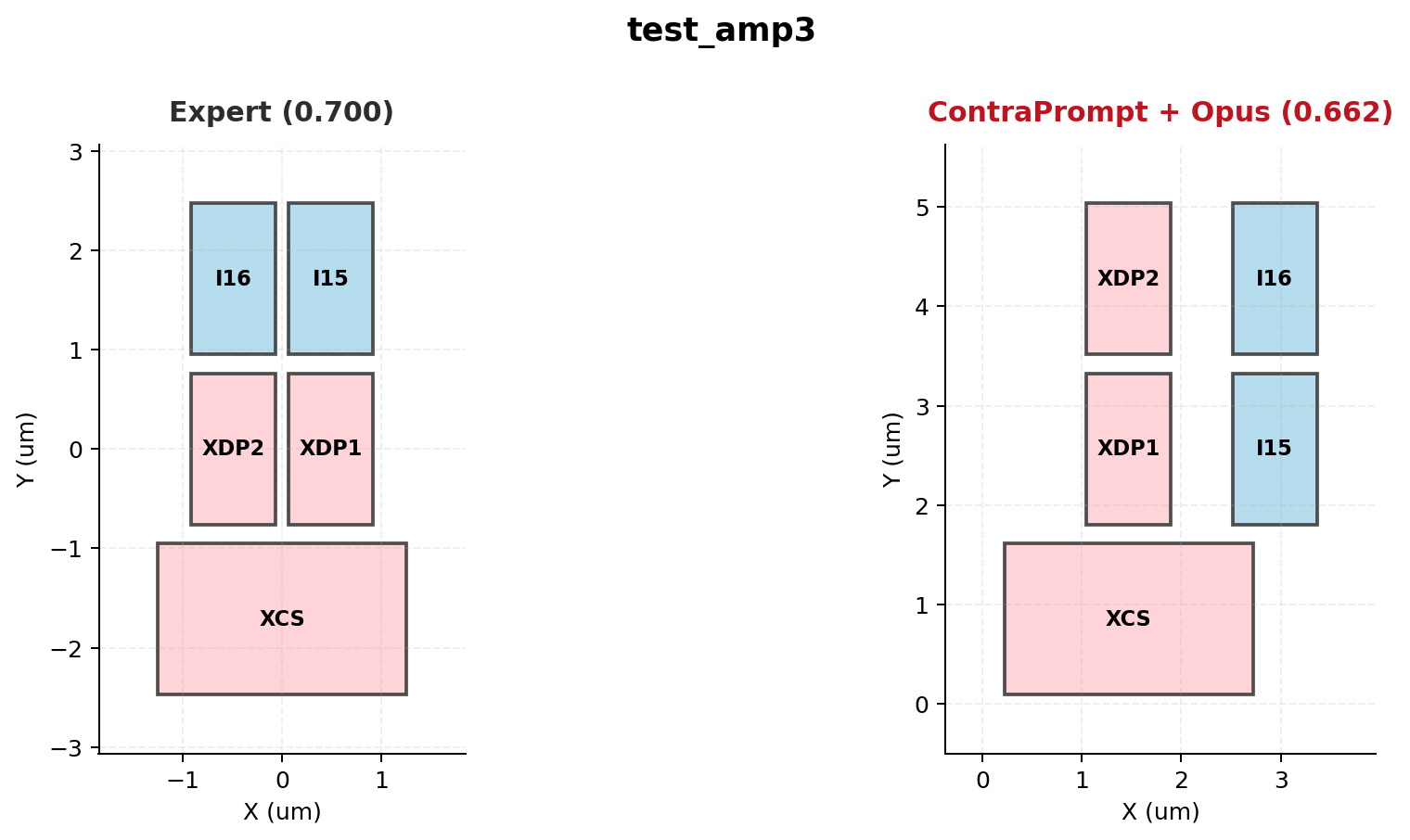 Figure 1: Average placement scores across 9 circuits. The gap between ContraPrompt+Opus (0.634) and Expert (0.652) is 0.018 — smaller than the gap between any two adjacent methods in prior work. TTT at 120B parameters scores 0.502, 26% below the prompt-optimized approach.
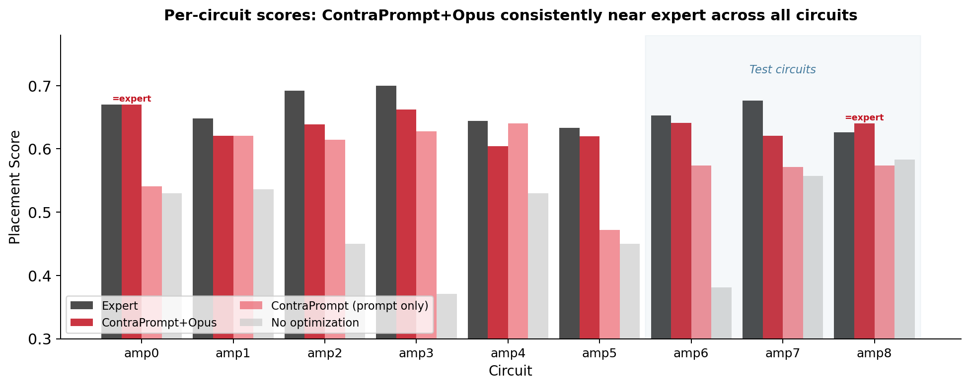 Figure 2: Per-circuit scores. The consistent gap between ContraPrompt+Opus and Expert across all 9 circuits (no circuit below 0.604) suggests the learned strategy generalizes rather than overfitting to specific topologies. The "No optimization" baseline shows high variance (0.371–0.583), indicating that the minimal prompt alone produces inconsistent strategies.
PromptGrad
PromptGrad evolves the prompt using textual gradients — at each step asking "what instruction change would have improved this placement?" We ran it on the same minimal prompt with abstract feedback (qualitative levels rather than specific scores, to prevent rules from hardcoding circuit-specific numbers). PromptGrad proposed rules across 3 epochs but none survived validation on our 6-circuit training set. We attribute this to the small dataset size: with only 6 evaluation circuits, the signal-to-noise ratio for gradient-based rule proposals is low, and rules that help on one circuit often hurt on another. On prior benchmarks with larger evaluation sets, PromptGrad converges reliably (see our CKTB results below where it finds the optimal in 2 attempts with feedback injection). This is a known limitation of gradient-based prompt optimization on small datasets — contrastive methods like ContraPrompt appear more sample-efficient because they extract rules from paired comparisons rather than aggregate gradients.GEPA
GEPA (evolutionary prompt adaptation with a stronger meta-optimizer) scored 0.556 on the diff amp benchmark — below ContraPrompt (0.624). During training, GEPA's evolutionary search developed a horizontal spreading bias visible in its reasoning traces: the model consistently pushes devices rightward even when vertical stacking would minimize wire length. On CKTB (below), GEPA converges to 0.595 while ContraPrompt and PromptGrad both reach 0.620 — the horizontal bias becomes a local minimum that the retry loop cannot escape. One explanation is that evolutionary search, by selecting across a population of prompt variants, can amplify layout priors that happen to correlate with score on the training distribution but don't transfer. Contrastive and gradient methods, which reason about why a specific placement scored poorly, appear less susceptible to this failure mode.Unseen Circuits
We evaluated all three optimizers on CKTA and CKTB with 10 attempts each and structured feedback injection between attempts.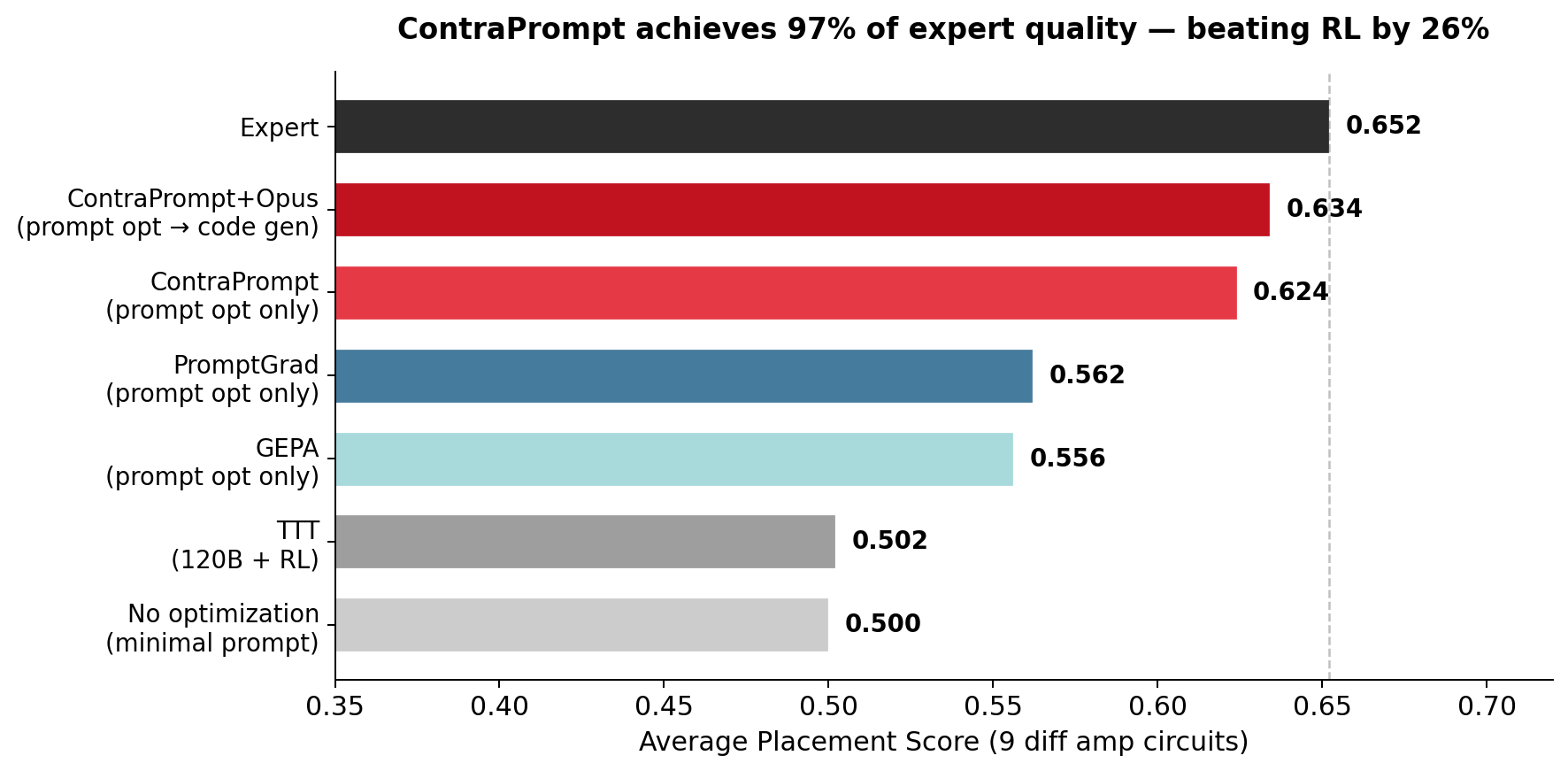 Figure 3: Cumulative best score across attempts. On CKTA, ContraPrompt converges at attempt 1; on CKTB, PromptGrad converges at attempt 2. GEPA plateaus at 0.595 on CKTB — 0.025 below optimal — due to its horizontal layout bias.
On CKTA, ContraPrompt reaches the optimal (0.628) on its first attempt. All three methods eventually converge to the same placement — identical coordinates for all 8 devices — but ContraPrompt requires 1 attempt vs. 4 for PromptGrad and GEPA.
On CKTB, PromptGrad reaches 0.620 at attempt 2, while ContraPrompt requires 7 attempts. CKTB's cross-coupled feedback creates multiple valid topologies; PromptGrad's learned search strategy navigates this space more efficiently than ContraPrompt's knowledge-driven approach.
We observe a consistent pattern: ContraPrompt converges faster on circuits with clear hierarchical structure (where domain knowledge directly constrains the search), while PromptGrad converges faster on circuits with feedback loops (where learned search heuristics outperform first-principles reasoning). Whether this pattern holds on a larger circuit set is an open question.
Figure 3: Cumulative best score across attempts. On CKTA, ContraPrompt converges at attempt 1; on CKTB, PromptGrad converges at attempt 2. GEPA plateaus at 0.595 on CKTB — 0.025 below optimal — due to its horizontal layout bias.
On CKTA, ContraPrompt reaches the optimal (0.628) on its first attempt. All three methods eventually converge to the same placement — identical coordinates for all 8 devices — but ContraPrompt requires 1 attempt vs. 4 for PromptGrad and GEPA.
On CKTB, PromptGrad reaches 0.620 at attempt 2, while ContraPrompt requires 7 attempts. CKTB's cross-coupled feedback creates multiple valid topologies; PromptGrad's learned search strategy navigates this space more efficiently than ContraPrompt's knowledge-driven approach.
We observe a consistent pattern: ContraPrompt converges faster on circuits with clear hierarchical structure (where domain knowledge directly constrains the search), while PromptGrad converges faster on circuits with feedback loops (where learned search heuristics outperform first-principles reasoning). Whether this pattern holds on a larger circuit set is an open question.
Placement Examples
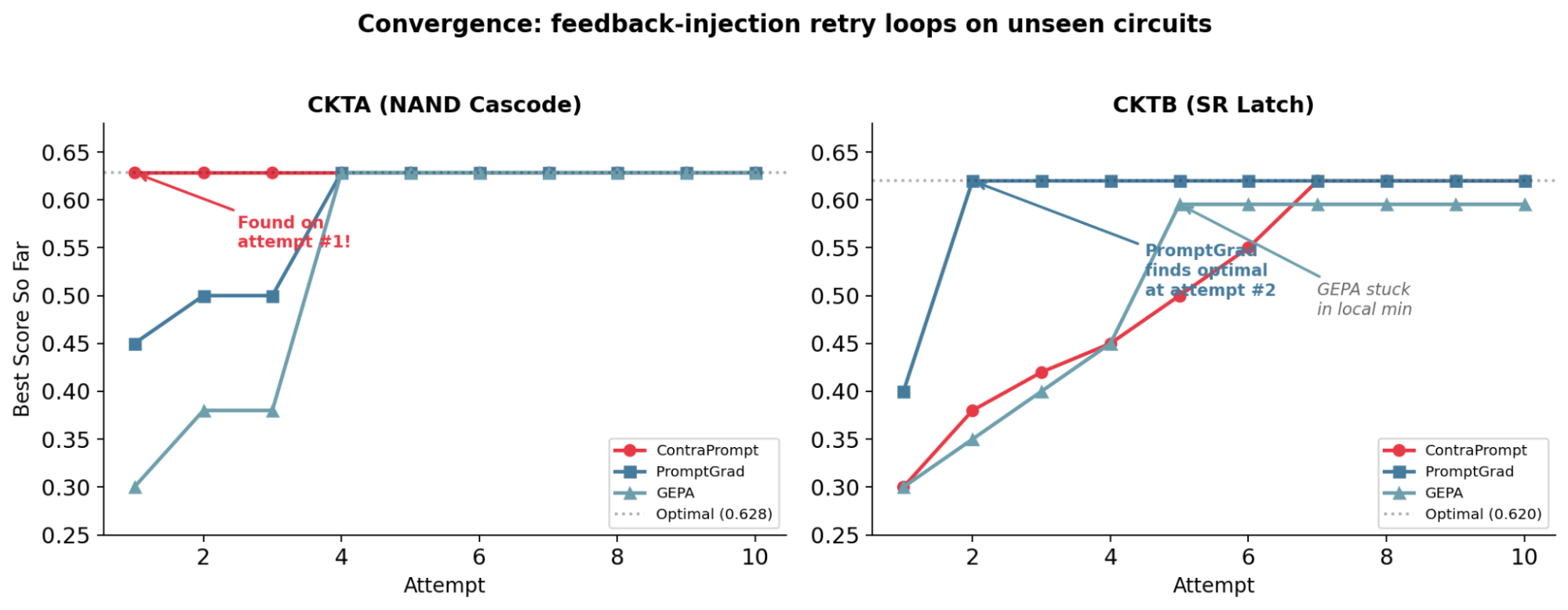 Figure 4: test_amp0 — Expert (0.670) vs. ContraPrompt+Opus (0.670). Both use a two-column layout with NMOS differential pair and tail current source in the left column, PMOS loads in the right.
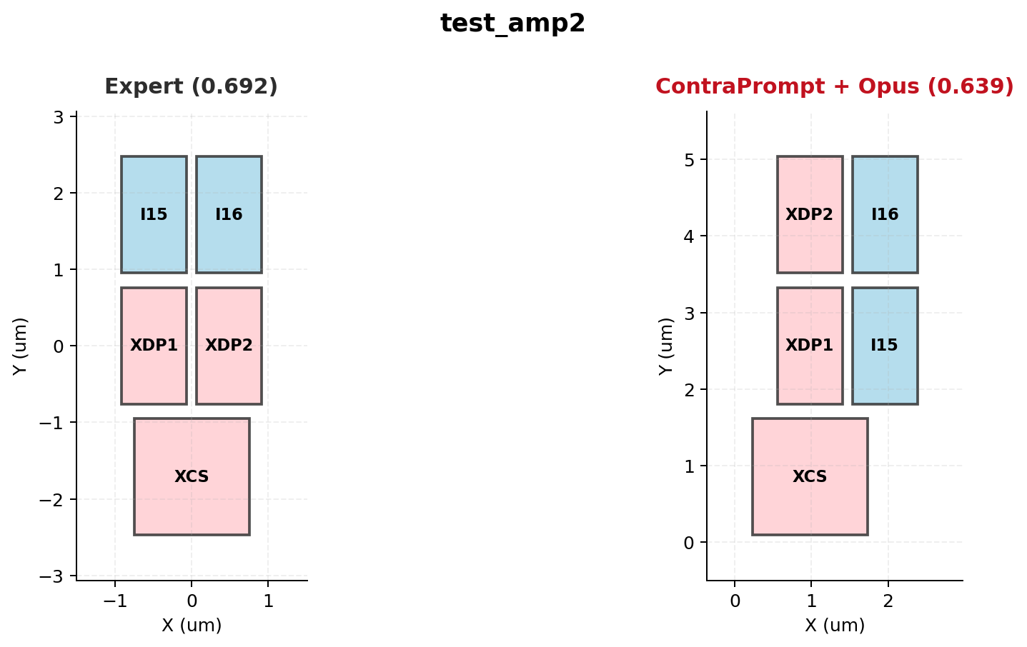 Figure 5: test_amp2 — Expert (0.692) vs. ContraPrompt+Opus (0.639). The LLM preserves differential pair symmetry and type separation but uses slightly wider column spacing, accounting for the 0.053 gap.
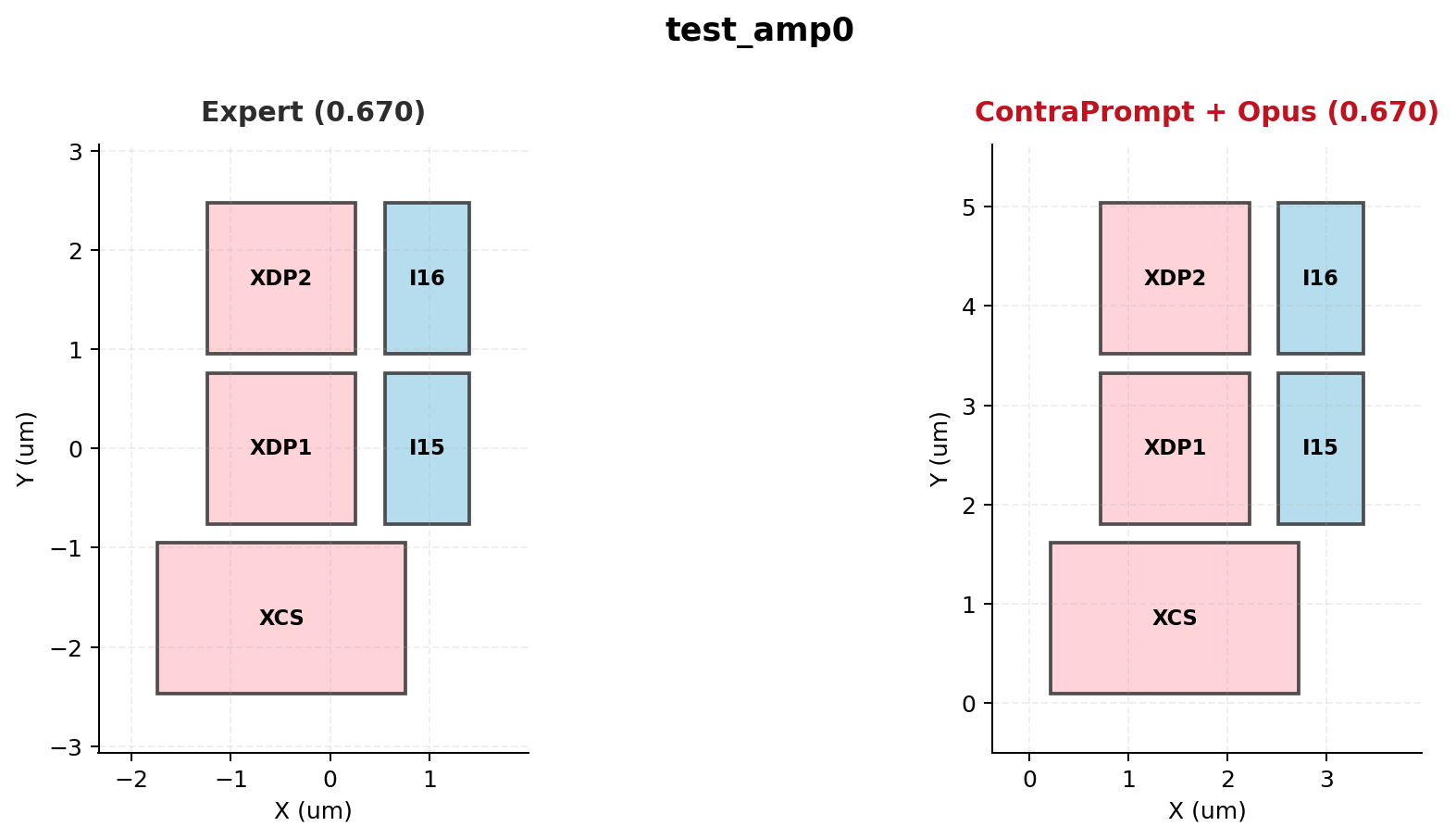 Figure 6: test_amp3 — Expert (0.700) vs. ContraPrompt+Opus (0.662). Device grouping is correct; the score gap comes from suboptimal vertical alignment of the drain-paired devices.
Summary
On 9 differential amplifier circuits, code generation with Opus reaches 97% of expert placement quality (test avg 0.634 vs. expert 0.652) with no training data or circuit-specific fine-tuning. The approach outperforms RL fine-tuning of a 120B model by 26% (0.634 vs. 0.502). Three observations from this work: ContraPrompt discovers domain strategy from scratch. Starting from a minimal prompt with no placement hints, ContraPrompt extracted column-based drain-pair alignment rules that improved Sonnet's scores by 24% (0.500 → 0.624). The rules encode high-level strategy rather than numeric parameters — the model fills in circuit-specific values at generation time. When paired with Opus for final code generation, the pipeline reaches 97% of expert quality. ContraPrompt and PromptGrad exhibit complementary convergence profiles. ContraPrompt converges faster on hierarchical circuits (1 attempt on CKTA) while PromptGrad converges faster on circuits with feedback loops (2 attempts on CKTB). PromptGrad's gradient-based approach struggled on our small 6-circuit training set, suggesting it requires larger evaluation sets to reliably propose rules. Whether an ensemble of both methods can capture the strengths of each is an open question. The 3% gap to expert quality likely requires finer-grained spatial control — per-device offsets, orientation-aware routing estimation, or multi-objective parameter search — rather than further prompt optimization.Want to try prompt optimization on your own use case? Try VizPy free or reach out to us.